Taxonomy of machine learning

Introduction

In the previous article of this series about machine learning, I tried to state clearly my understanding of machine learning. I argued that I understand machine learning as a set of algorithms and methods for automatically determining the parameters of mathematical models and automatically choosing the best fitting model for a given problem.

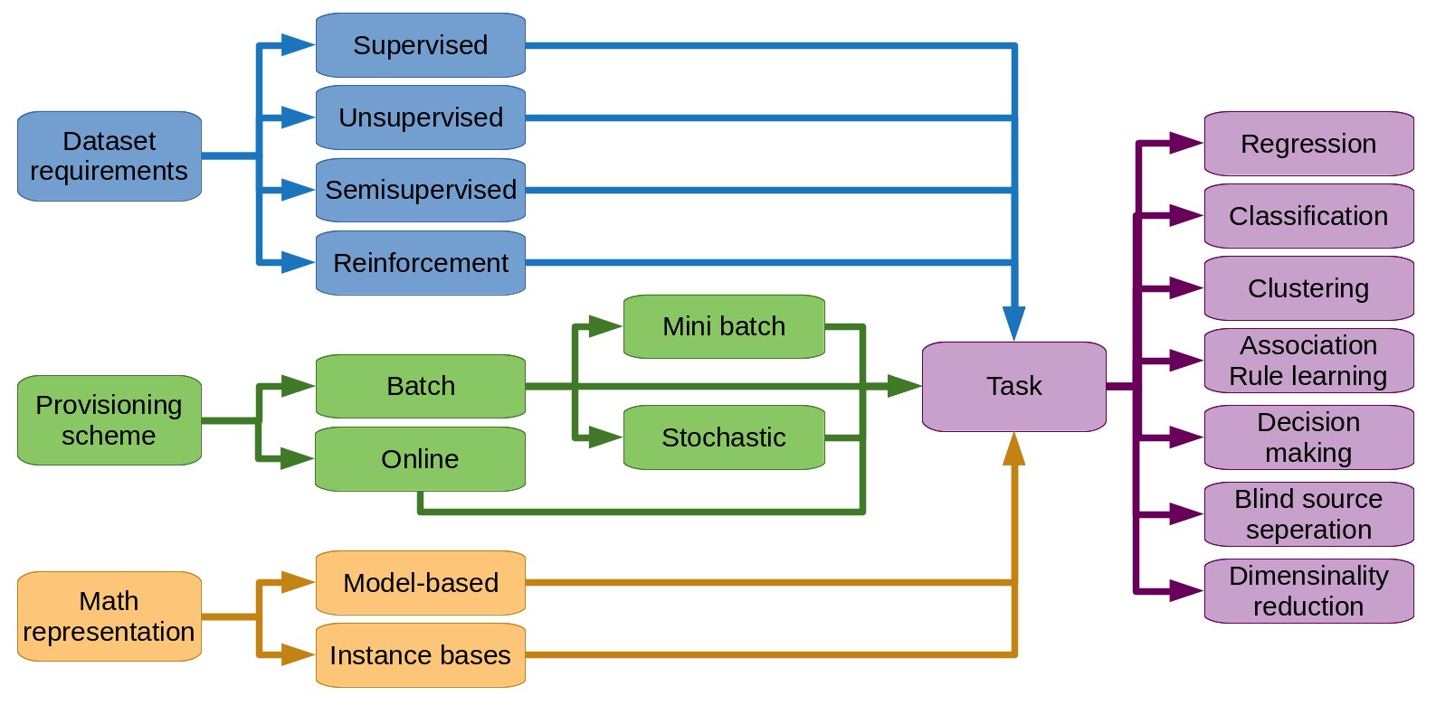
In this article I will try to briefly present my personal taxonomy (or categorization) of machine learning techniques. Hopefully, this will also give us an overview of the usages of machine learning.

Click the table of contents icon on the right to have a hierarchical view of the taxonomy at any moment. I also suggest to open the internal links in new tabs so that you don’t lose your reading position in the article.

Taxonomy by data set requirements

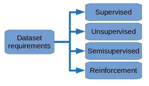
Depending on the data available and the objective of the software package we are developing, we will train our models differently. In the next sections, we discuss supervised learning where example outputs (expected results) are given, unsupervised learning where no example output is given, and reinforcement learning where learning occurs by interacting with an environment.

Supervised learning

A supervised learning algorithm requires the presence, at the training phase, of the correct expected output for each element of the initial data set. We say that the inputs are labelled.

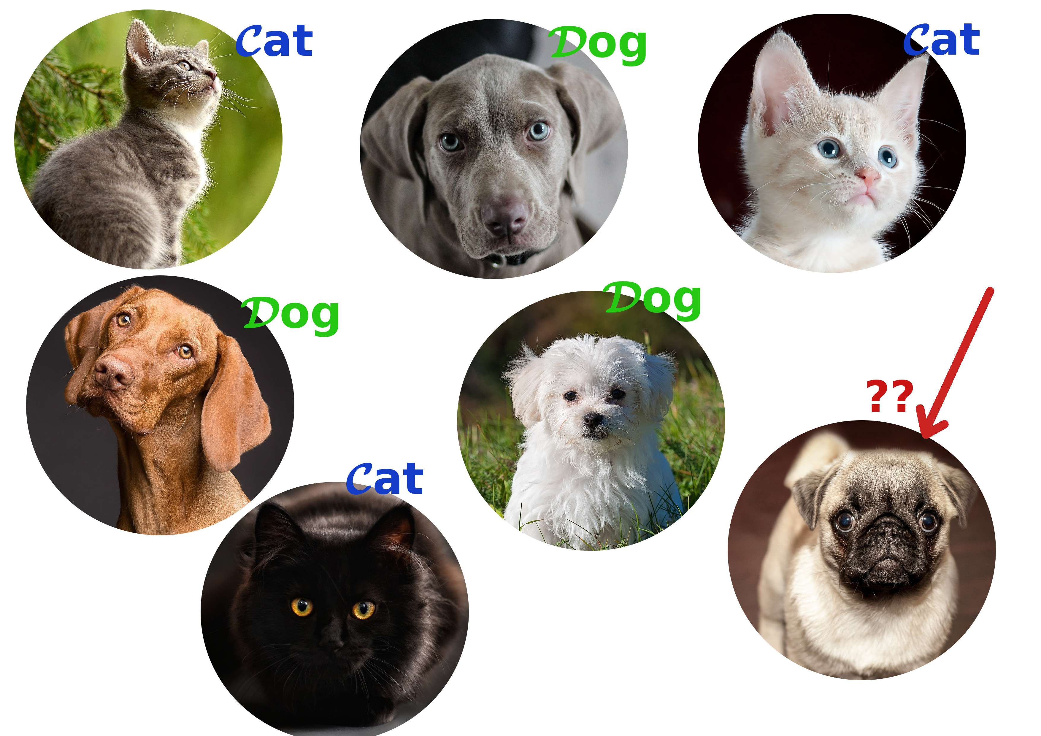Illustration of supervised learning. The algorithm can learn from the labelled images of dogs and cats. The image on the bottom right corner is the new input to be labelled.

For example, let’s suppose that my data set is my email box. Let’s suppose I use to manually sort my emails as “spam” or “not spam”. Now let’s suppose I want to create a program to automatically filters my emails for me. In this setting, I have examples to feed my learning algorithm with: the manually classified emails. So I have not only the inputs in my data set (the emails) but also the corresponding outputs (whether they are in the spam folder or not). An algorithm that relies on such a data set is called supervised. It requires input values and their corresponding outputs. From these examples, it will determine the best prediction function to estimate the outputs for new inputs.

An analogy of supervised learning is often cited as the situation where we show an object to a child and we say the name of that object so that the child learns to name the object.

Unsupervised learning

Unlike supervised learning, an unsupervised technique does not require example outputs (or labels).

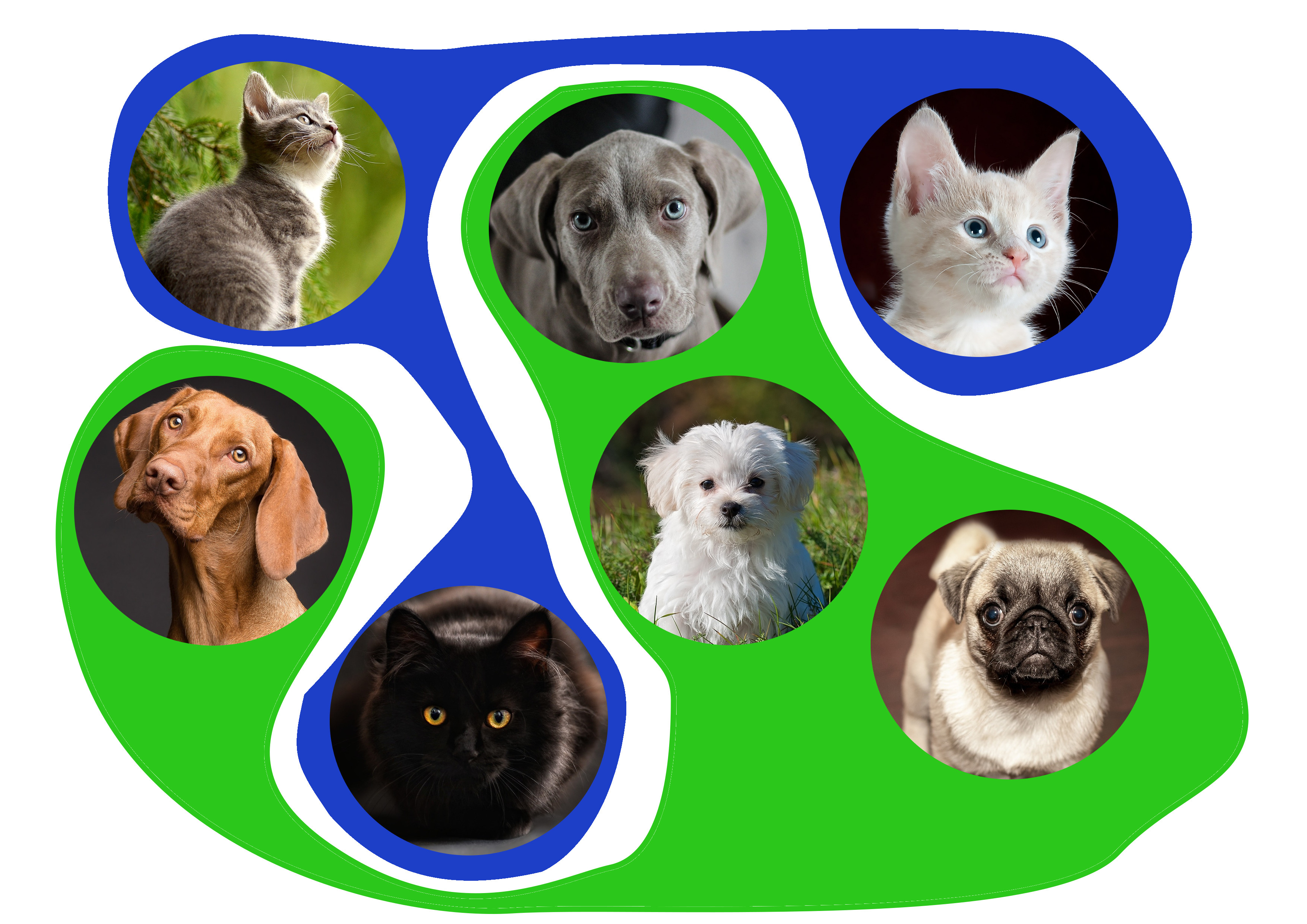Illustration unsupervised learning. The colored areas show the grouping of unlabelled images of dogs and cats. The algorithm groups together images with similar features.

For instance, let’s assume that I have a database that contains the sales history of customers on an online shop over a decade. Let’s suppose I want to create a recommender system for this shop. My goal is, given a product that a customer is currently viewing, to suggest another product that has the maximum chance to be bought along with the one being viewed. For example, intuitively, I may suggest baby diapers if a customer is viewing a baby bottle. I want my learning algorithm to automatically discover this kind of associations in my dataset.

In this example, I didn’t have any correct output to train my algorithm with. I only had the inputs, i.e. the transactions in the database. Below we discuss association rule learning, a set unsupervised learning techniques designed to extract this kind of relationships from a data set of transactions.

Semi-supervised learning

I see semi-supervised learning as an unsupervised learning extended by a supervised learning.

Semi-supervised learning is typically used when we have a small amount of labelled inputs and a much larger amount of unlabelled inputs.

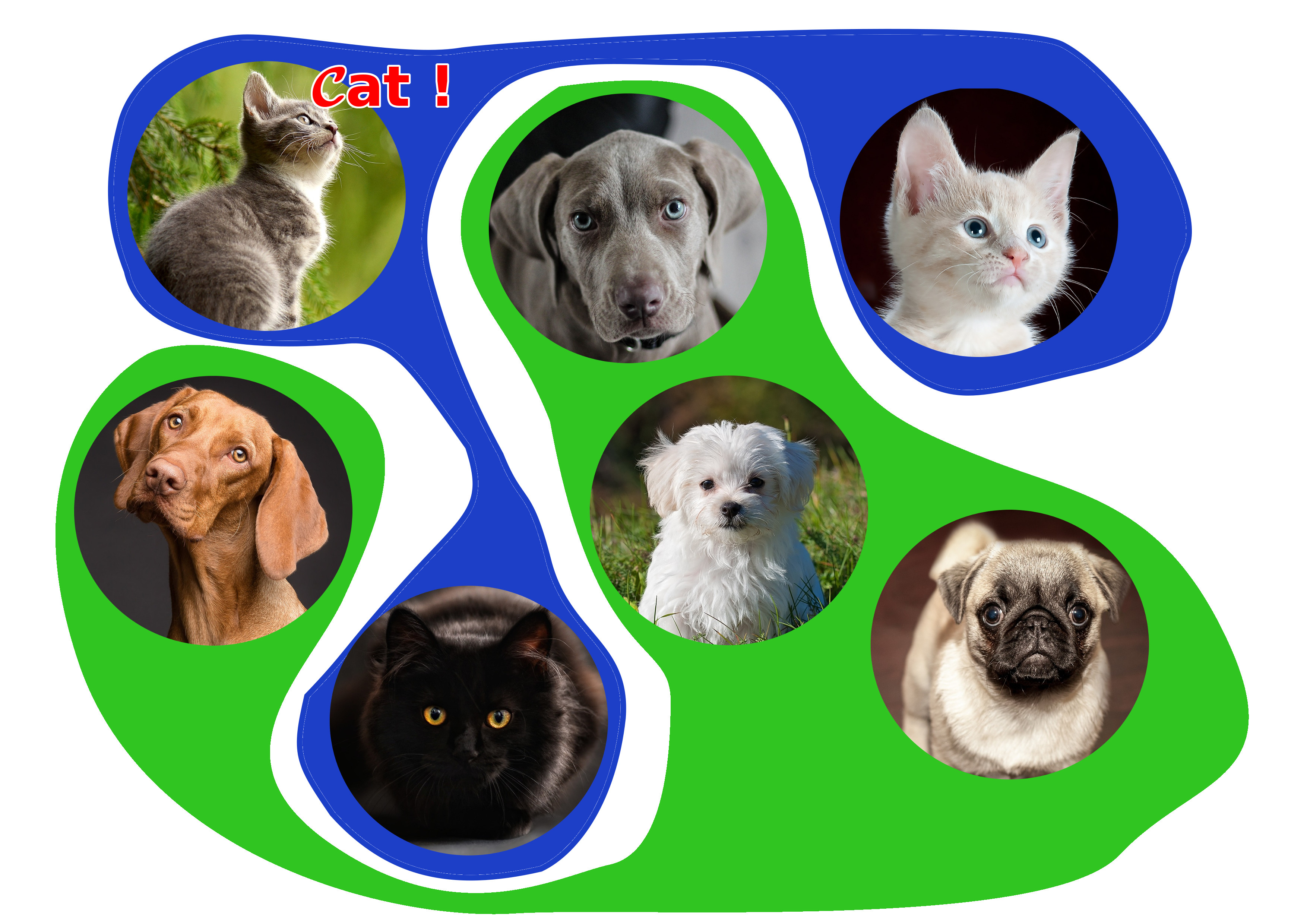Illustration of semi-supervisered learning. An unsupervised phase groups unlabelled images of dogs and cats (colored areas). A supervised phase, using the unique labelled image in the top left corner, can then label all cats as "cat", and all dogs as "not cat".

For example, let’s reformulate our email filtering example such that I only have $20$ emails over $20 000$ that are sorted into $2$ folders as spam or not spam. Most supervised learning algorithms trained on just the $20$ emails will perform poorly on the much larger set of unsorted emails. One solution may be to run an unsupervised algorithm that will group similar emails ($2$ groups in our case). This grouping algorithm is applied on the complete data set ($20000+20$ emails). Then we would assign to any unsorted email the folder of its closest neighbour (according to some metric) among the $20$ sorted emails that lies in the same group. More clearly, let’s denote an email by a number ranging from $1$ to $20020$ where $1$ to $20$ denote the sorted emails. If for instance email $2$ (which is among the $20$ sorted emails) has the shortest distance from any email denoted $i$ and email $2$ is a spam, then we would consider email $i$ to be a spam as well.

In this example we actually used two unsupervised algorithms: the first one to create the groups is a clustering algorithm and the other one to find the nearest neighbours is a classification algorithm, 2 taxons that we’ll discuss a few sections later.

I shall mention that some authors have the inverse point of view - seeing semi-supervised learning as a supervised learning extended by an unsupervised learning - where the unsupervised learning can be seen as a preprocessing.

Finally, we will note that semisupervised learning is often used in configurations where collecting data is cheap but labelling is expensive (generally time-consuming).

Reinforcement learning

Reinforcement learning does not require an initial data set, but rather an environment (or context). Data is collected by the learning algorithm by exploring the environment. The algorithm tries to optimize a decision process toward a goal.

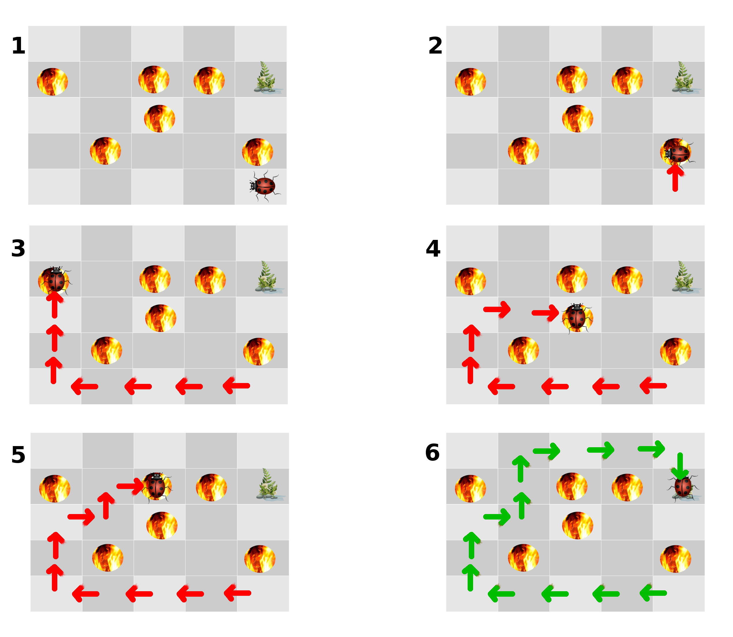Illustration of reinforcement learning. The algorithm explores the environment and learns how to get to its goal (attained in picture 6).

Problems for reinforcement learning include optimizing the behaviour of autonomous agents, decision making for stock market investments, route optimization, game strategy, business strategy and more.

Taxonomy by mathematical representation

Some machine learning techniques simply compare new instances to the ones they were trained on. Other techniques try to find a general representation of the relationships in the dataset. The first are called instance-based and the latter model-based.

Instance-based learning

In order to make estimations, a predictor trained by an instance-based learning algorithm compares new data to the training examples.

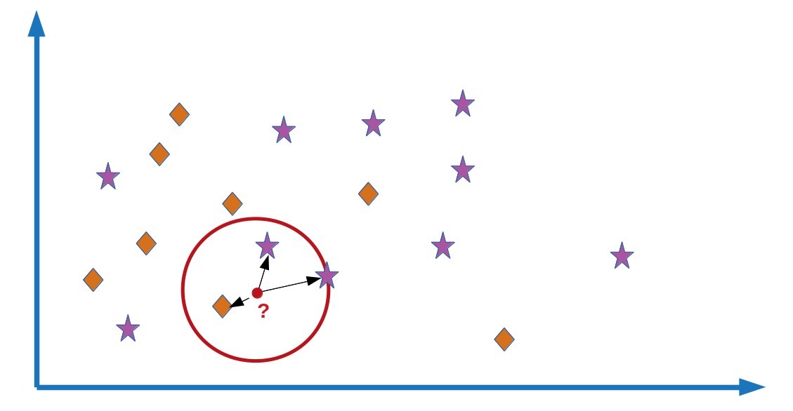Illustration of instance-based learning. The red dot is the "new" input to classify. Its closest neighbours lie in the red circle. It will be classfied as "star" because this label if the most common among its closest neighbours.

Generally a distance metric or sometimes a similarity measure is needeed. Distance metrics include the Euclidian distance, the Hamming distance, the Levenshtein distance (used for text comparison), etc.

Strategies to estimate the property of interest for new data include “voting” and averaging. Voting means that the algorithm’s estimation will be equal to the most common value among the $k$ training examples that are the closest to the new data (according to the chosen distance metric). Averaging means giving as our estimation the average value of the property of interest of these $k$ closest neighbours. In the case of averaging, if $k=1$ then we just give the value of the closest neighbour as our estimate.

In our example of a semisupervised learning email filtering, the unsupervised phase where we sorted the $20000$ unlabelled emails by “just comparing” them to the $20$ labelled emails is an example of an instance-based technique.

Model-base learning

A model based-learning algorithm tries to generalize from the training examples. The mathematical representation that the algorithm obtains from this generalization process is the model that it will use to make its estimations on new data.

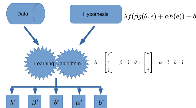Illustration of model-based learning. The algorithm chooses an hypothesis, a mathematical representation. Then it determines the parameters of this hypothesis based on the available data.

Our discussion on getting an intuition of machine learning gave us (hopefully) a good sense of what learning a model is.

Taxonomy by training data provisionning scheme

Intuitively, we sense that machine learning techniques should not have a memory of the entire dataset they were trained on. However, the iterative ajustements that the learning technique does on the mathematical representation it is determining are based on the data it is provided with. For these antagonist reasons, we can intuitively understand that many learning techniques will not be able to adjust on new data an already trained representation while keeping it consistent with its previous training (because there is no memory of the previous data).

Learning techniques that require the entire data set for their training are called batch learning methods. Some learning algorithm can actually adjuts an already trained representation to new data. They are called online learning methods.

Batch learning

In batch learning, all the examples must be provided during the traning phase. The “predictor” resulting from the training is then used in production and no more learning occurs.

In this setting, if we obtain new examples, we need to train a new model from scratch on the complete enriched data set.

For large data set that cannot fit entirely in a computer’s memory, some techniques exist to cope with batch learning. They are called out-of-core methods. Some of them address the issue at the data access and management level, allowing for example to load in memory only the part of the data require for a calculation at time $t$. They usually transform the dataset into a new representation that facilitates these optimizations. Other methods are variants of batch learning to accept the data by small chunks. Mini-batch techniques still require the entire data set at training time but “consume” data by small subsets. Stochastic methods consume one element at a time and pick this element according to a probability distribution.

Online learning

Unlike batch learning, an online learning technique can be provided with new training examples progressively and changes its representations accordinly, even while being used in production.

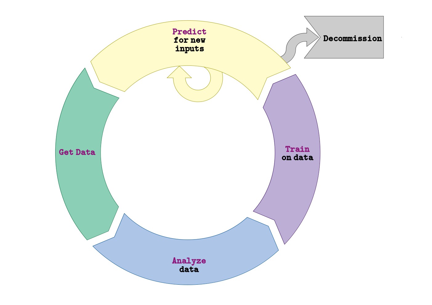
An online learning algorithm takes the current best predictor as an additional input.

For many underlying representations, true online learning is not possible. However, depending on the formulation, we can often find a pseudo online algorithm based on recursive algorithms. In this case, the new predictor depends on the current best predictor and all the previous examples (already learnt). On lucky cases the dependency on previous examples can be expressed using an aggregation function. In this case, we do not actually store these data elements but rather the aggregation function and the information needed for its computation (including its previous result). When no such trick is possible, then no guarantee can be given about the storage or memory complexity of recursive pseudo-online algorithms.

Taxonomy by usage or goal

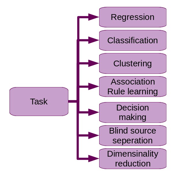
Common machine learning tasks include:

• Finding the value of a property of a phenomenon that depends on other properties of this phenomenon (or other instances). This task is called regression.

• Finding boundaries to seperate data elements into groups. When the groups are imposed from the beginning (they are part of the inputs of the algorithm), the task is called classification, when the groups are to be discovered by the algorithm we call the task clustering.

• Optimizing decision processes.

• Mining association rules (association rule learning).

• Disassembling a measurement (usually a time series) into its basic independent components. This is blind source separation.

• Reducing the number of input variables of a learning problem, a.k.a dimensionality reduction.

Regression

Illustration of regression. The input data has only 1 feature. On the left, a degree 3 polynomial regression and on the right a linear regression.

Regression tries to find the value of a property of a phenomenon depending on the values of other properties or instances of the same kind.

Regression typically falls under supervised learning.

For example, suppose an ice cream seller wants to predict its incomes based on temparature forcasts. We would be learning the (model and) parameters of a regression if we were to try to create a software package for this requirement.

Classification

Classification tries to find boundaries in the dataset so as to seperate the elements into a number of classes known (or defined) before the training.

Illustration of classification. Both of the models illustrated above draw linear boundaries (the data is linearly seperable). Credit: [1]

Classification typicaly fall under supervised learning. However there exist unsupervised classification, like anomaly detection or outliers detection.

For example, if we had a labelled data set consisting of pictures of handwritten digits ranging from $0$ to $9$, training an algorithm to recognize the digits on new pictures would be a classification task where the classes are $1, 2, \dots, 9$. Moreover, our emails filtering example is a classification task with two classes: spam or not spam.

I see classification as a different beast from regression but some authors present them as two similar tasks. For these authors, the only conceptual difference is that the output of regression is continous while the output of classification is discrete. I don’t share this vision, because as stated above I see regression as trying to estimate a value while classification tries to estimate a boundary.

Clustering

Clustering tries to group observations such that elements belonging to the same group (or cluster) are more similar - according to some similarity measure - and thoses belonging to different groups are more dissimilar.

Illustration of clustering. The plotting represents the clusters with colors. Credit: [2]

Clustering typically is an unsupervised learning task.

We presented clustering while talking about semisupervised learning through our modified example of email filtering. In the real life, clustering helps biologists in creating their taxonomy, marketers in finding groups of customers sharing similar behaviour, search engines in categorizing web pages…

Decision making

Decision making tries to find which decision to take so as to optimize a gain, the usage of a resource or an evolution toward a goal.

Illustration of reinforcement learning. By exploring the environment, the algorithm learn which decisions to take in order to attain its goal.

Optimal decision making can be learnt using any of supervised, semisupervised or reinforcement learning. It is however often associated with reinforcement learning.

Machine learning for decision making is used for trading on stock markets, building autonomous agents (like planet Mars rovers), making decisions in politics, insurance and many more domains where strategy is important.

Association rule learning

Association rule learning tries to determine how actors associate items.

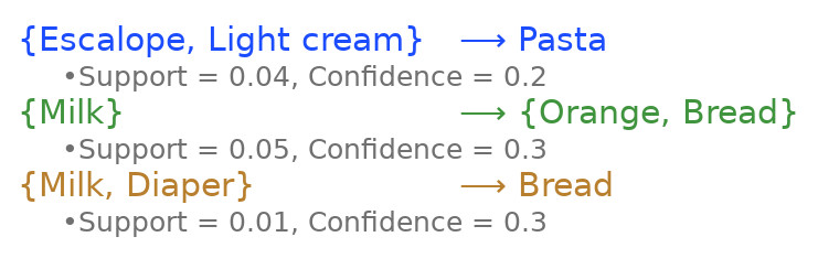Illustration of association rule learning. The rules on this example represent the associations of products often present in customers carts in a shop. Customers buying milk and diapers often buy bread :)

The fundamental conceptual difference with clustering, in my opinion, is that the grouping of clustering is based on the properties of the elements while association rule learning is based on how other agents or actors group elements together in some transactions.

Association rule learning is typically based on unsupervised learning techniques.

We gave an example of association rule learning when we discussed unsupervised learning above. Other usage of algorithms resulting from association rule learning include ordering books in a library, placing products in a shop, composing service packs (for insurances for example)…

An analogy for association rule learning is how we decipher an ancient language. Knowing the basic common structures of languages, their relationships to one another (ancestry, similarity…), other statistical properties and some historical facts, we learn the association rules used by the ancient users of the language so that the scripts they left make sense to us.

Blind source separation

Blind source separation tries to decompose a measurement into its basic components. Generally the measurement is a time series, like a sound record.

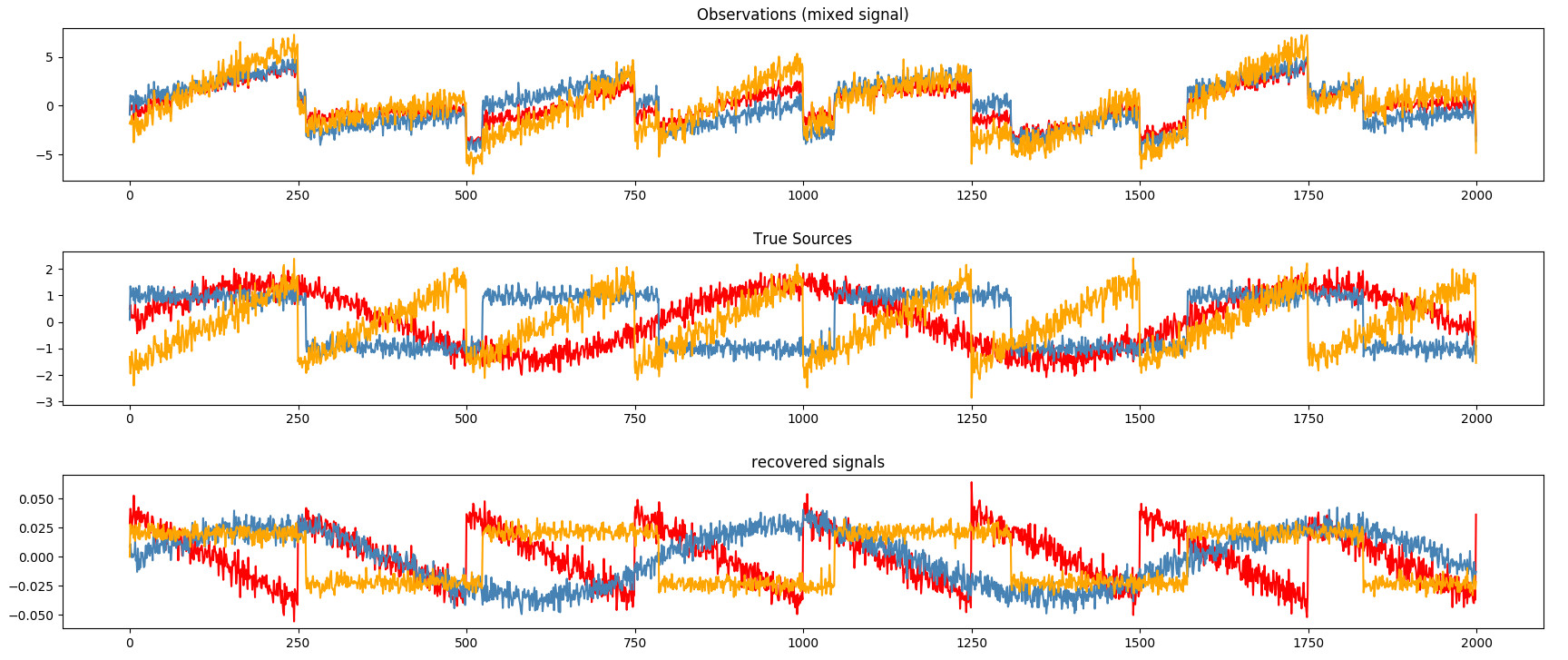Illustration of blind source seperation. The signals are correctly recovered (bottom image), but the colors differ. This illustrates the "blind" aspect of the algorithm, which actually knowns nothing of the initial signals (middle image). Credit: [3]

Blind source separation is typically an unsupervised task, but it can be supervised as well.

An often cited example of blind source separation is detaching the speeches of different persons from a recording where they all talk at the same time. Let’s imagine we are at a party and get to the kitchen where there are 5 people talking at the same time. We make a record of this cacophony and we latter want to seperate each person’s speech to a seperated track. This would be a task for blind source separation. Here “blind” means that the algorithm has no information about the sources of the signals neither about the mixing process.

An analogy of blind source separation is how we humans, in a crowd with several people speaking, are able to isolate the voice of someone in particular that we want to listen to.

Dimensionality reduction

Dimensionality reduction tries to reduce the number of input variables of a learning problem while keeping as much relevant information as possible.

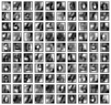Illustration of dimensionality reduction. Each image represents a hand-written digit. Both feature selection and extraction gave these grayscale pixellate images. The classification algorithm appends to works very well on the reduced dataset. Credit: [4]

The output of dimensionality reduction can be used as input of other learning algorithms or for visualization (if the number of inputs can be reduced to $3$ or less). When used as input of other learning algorithms, it can improve their performances (reduce their generalization error) because less variables often means less complex learning algorithms, less noise and less redundancy in the data.

The input variables of learning algorithms are called features. Usually, dimensionality reduction consists in 3 types of reduction of features:

• Feature selection tries to find a subset of features that are most relevant for a given problem.
• Feature extraction is often used in conjunction with feature selection and tries to infer new features from the existing ones. These new features will hopefully be more informative and less redundant than the initial ones and still accurately describe the initial data set.
• Feature projection reduces the dimension of the inputs by projecting them onto a lower dimensional “geometry”. Feature projection is useful when we suppose that the inputs are described by a lower dimensional “geometry” but folded in a higher dimensional space. For example, in the picture below, the S shaped inputs on the left make a 2D surface “folded” in a 3D space.

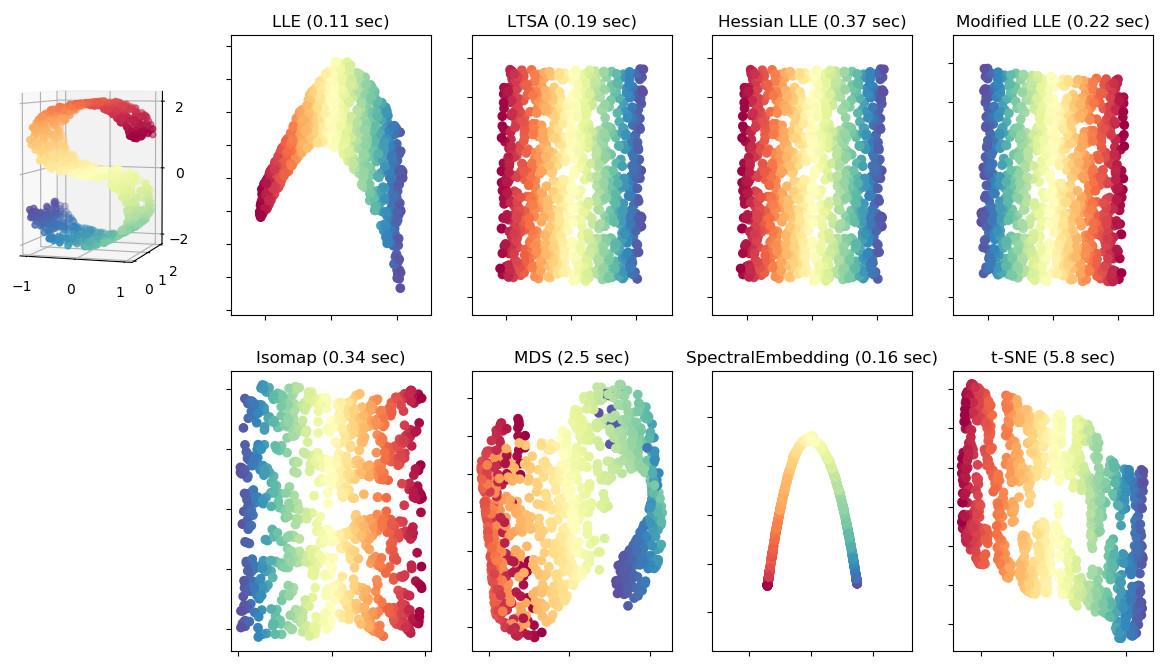Illustration of feature projection. Various projections onto a plane of a 2D surface folded in a 3D space. Credit: [5]

We should note that a big challenge in machine learning is sometimes finding or choosing the representation of our features. For instance, in the example of the email filtering, how could we represent an email numerically such that it can be a relevant input for a learning algorithm ? One method may be to: 1) create a “dictionary” that contains all the words that appear in all emails, 2) represent an email by a vector where each component is the dictionary’s indice of the email’s word. Another option maybe that each component of the vector is the number of occurences in the email of each word of the dictionary. Other representation are possible.

A basic illustration of dimensionality reduction can be seen in our example of digit recognition from the section on classification above. Maybe we didn’t need color informations in order to recognize the digits, so we could drop $2$ color components and reduce the dimensionality of our data from $3$ (R, G, B channels) to $1$ (grayscale value). In the same idea, we can reduce the size of the image and compress it to even more reduce its dimensionality.

Let’s consider another example: a program that says whether a picture shows a face or not. We humans just need a few lines of drawings in order to recognize a face, so we might intuitively think that our algorithm also need only a small amount of the informations from a picture to tell whether it is a face or not. There actually exist neural networks capable of extracting such features from an image and that allow other algorithms to classify the image as face or not face.

Conclusion

There was a lot of informations in this article, so let’s recap.

There are different axes of taxonomy of machine learning algorithms.

We can differentiate machine learning techniques based on the kind of data they require in order to learn. In this taxonomy we distinguished supervised, semi-supervised, unsupervised and reinforcement learning.

Another axis of taxonomy is the mathematical representation they rely on. From this axis we distinguished model-based and instance-based learning techniques.

A third alternative of differentiating machine learning algorithms is by the way they consume data for training. In this axis we have batch and online learning methods.

Finally, we can base our taxonomy on the type of task the algorithm resulting from the training tries to achieve. These tasks are notably regression, classification, clustering, decision making, association rule learning, blind source separation and dimensionality reduction.

These axes of taxonomy are not exclusive. For example, a supervised learning algorithm can be an instance-based and an online learning technique. Moreover, the taxonomy presented in this article is my personal attempt in linking various qualifications of machine learning techniques, and it is not exhaustive.

Taxonomy is useful when we try to frame a problem and try to determine which learning technique to use for this particular problem. Knowing these taxonomies can guide us in finding a reduced subset of candidate learning algorithms among which a validation technique (for example) can choose.

In the next article, by discussing linear regression, we will make a big step toward actually applying machine learning in practice.

Credits

• [1]: Scikit learn - Multilabel classification
• [2]: Scikit learn - Demonstration of k-means assumptions
• [3]: Scikit learn - Blind source separation using FastICA
• [4]: Scikit learn - Restricted Boltzmann Machine features for digit classification
• [5]: Scikit learn - Comparison of Manifold Learning methods

Written on Sun Jan 13th 2019, 11:00 GMT+00:00.
Last updated on Sun Mar 10th 2019, 11:18 GMT+00:00.